US South Pine Pulpwood Price Dynamics

In economics, elasticity is a measure of responsiveness. How does price respond to an increase in demand or an increase in supply? How does demand respond to an increase or decrease in price? Economists use price elasticity to determine how suppliers or buyers of a product respond to changes in that product’s price. Typically, price elasticity is calculated by dividing the percent change in the quantity of supply or demand by the percent change in price.

Supply or demand for a good is inelastic when its price calculation is less than one; this means that changes in price for that product have a relatively small effect on the amount of demand for that product. Zero indicates that a product is perfectly inelastic, meaning that changes in price have no effect on supply or demand. The supply or demand for a good is elastic when its price elasticity is greater than one; this means that changes in price have a relatively large effect on the amount of supply or demand for the product.

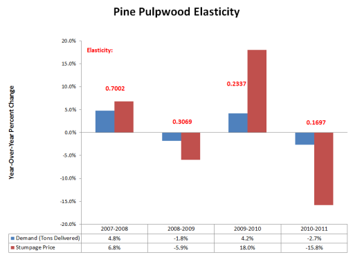
At Forest2Market, we often calculate the price elasticity for forest products when analyzing supply and demand changes in local wood baskets and when forecasting long-term price reactions. One recent study revealed the following price elasticity of pine pulpwood demand for the US South from 2007-2011:

• 2007-2008 = 0.7002
• 2008-2009 = 0.3069
• 2009-2010 = 0.2337
• 2010-2011 = 0.1697

Detailed measurements for these calculations can be observed in the trend chart to the right (Figure 1). Price changes for pine pulpwood are stumpage price changes calculated from our online stumpage database. Demand changes for pine pulpwood are sourced from our mill receipt data (tons purchased) collected through our delivered pricing service, Forest2Mill^®.

Figure 1

As you can see, pine pulpwood demand and pricing have experienced ups and downs over the last few years. Most notable is the change during 2011, when demand decreased 2.7% and stumpage prices decreased a whopping 15.8%, over period. Though pine pulpwood prices were relatively inelastic throughout the entire period, they were the most inelastic in 2011.

So what were the drivers of the extremely low elasticity rate in 2011?  A combination of two factors:

End-Product Demand and Risk – Despite high unemployment, real US GDP grew 1.7% from 2011 over 2010. In addition, despite the recent chaos in the Eurozone, real GDP there grew 1.5% over the same period. During this time period, an additional 2.4% of wood fiber moved through mills in the US South. This points to a slight increase in demand for pulp products in 2011 over 2010. However, we also observed that wood fiber inventories at mills in the South increased 16.0% over the same period.

Looking at US South precipitation, total precipitation fell 27% in 2010 from 2009’s high, and then increased by just 2% in 2011. Because these precipitation levels allowed for more harvesting activity, mill inventory levels returned closer to their historical norms. This reduced the risk that mills would run out of wood fiber.

But what gives?  If mills are increasing production and building inventory, shouldn’t they be consuming more pulpwood?

2. The answer to that last question is that the supply of residual chips from sawmills has increased, and pulp producing mills purchased more chips and less pulpwood. As the housing market grew by 5.8% in 2010 and 4.4% in 2011 over 2010, sawmills increased production by 13.5% and 10.3%, respectively (Figure 2). As a result, residual chip production increased 7.4%. (On a side note: the increased activity in the lumber market did not translate into higher lumber prices or pine sawtimber prices for 2011. Lumber prices actually retreated over the period. See Mike Fiery’s blog post on this effect on pine sawtimber prices.)

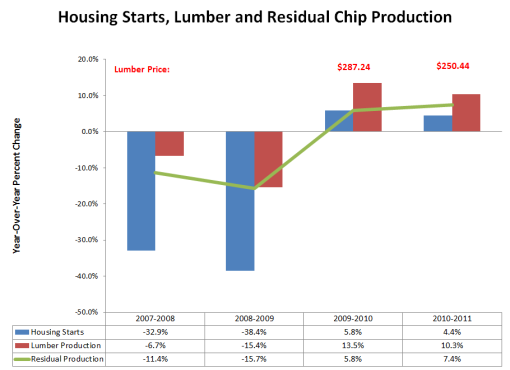
Figure 2

The end result was a 15.8% reduction in pine pulpwood stumpage prices. For timberland owners, the higher pine pulpwood prices in 2010 were a bright spot compared to stagnant prices for pine sawtimber. With the exception of moving a little more sawtimber volume in 2011 due to increased sawmill demand, timberland owners are struggling to find value-add in the market. For pulp mills, both cost and risk dramatically improved in 2011.

Looking into 2012, we’ve observed little change through the first half. Local pockets like southeast Georgia/northeast Florida are exceptions. Southwide, we expect to see slight increases in sawtimber prices and the continued depression of pine pulpwood prices.

Comments

US South Pine Pulpwood Price Dynamics | F2M Market

07-01-2012

[...] US South Pine Pulpwood Price Dynamics | F2M Market Watch. Share this:ShareTwitterFacebookLinkedInTumblrStumbleUponPinterestLike this:LikeBe the first to like this. [...]

Comments

Tim Sydor

07-03-2012

Daniel -

In economic literature price elasticity of demand is negative. The primary reason - demand curve (and the elasticity is movement along the demand curve) is downward-sloping. As you write: “Typically, price elasticity is calculated by dividing the percent change in the quantity of supply or demand by the percent change in price.” And that is not what you calculated, right? In economics the price is an independent factor, but quantity (at the individual level) is a dependent factor. Market participants are generally assumed to be price takers, one of the results/requirements of competitive markets. And it is usually assumed that, since it is a movement along a single demand curve (short-term) other factors, e.g. lumber prices, housing starts, unemployment are fixed.

What you did was to take a log of delivered price on a log of delivered volume, one way of doing elasticity, which is in effect an invert of the formula stated in “Typically,...”. Technically it is a “demand elasticity of price” and it attempts to answer your question: “How does price respond to an increase in demand or an increase in supply?”. What you seem to capture is not movement along the demand curve (as price elasticity of demand does), but a movement along a market-clearing equilibrium points of many individual demand curves. Each is shifted left-right based on various exogenous factors (GDP, lumber price, etc.). In effect it is a movement along a long-term (in economic sense) supply curve.

Other thoughts: stats for your 2007-2008… calculations would be nice. Are they even statistically significant? In explaining two drivers of extremely low elasticity you state #1. What is # 2?

Comments

Allen Waddell

04-07-2013

Dear Sir: For the last 50 years the landowners in Georgia have had a negative return on timberland.We sold pulpwood last year in hancock county for $3.00 a cord. Land is $2800.00 an acre. at 10% interest and 10 year mortgage equals $560.00 a year, $30.00 in taxes, $100.00 management total is $690.00 Vs. two cords of growth x $3.oo equals $6.00 income, loss equals $684.00 a year. Allen Waddell